2 Data

2.1 Description

For this project, we will use historical stock data for companies in three key sectors: Technology, Finance, and Healthcare. The dataset will span five years, allowing for a robust analysis of trends over time.

2.1.1 Sectors and Companies

2.1.1.1 Technology:

Apple Inc. (AAPL)
Alphabet Inc. Class C (GOOG)
Meta Platforms Inc. Class A (META)
Microsoft Corp. (MSFT)
NVIDIA Corporation (NVDA)

2.1.1.2 Finance:

Bank of America (BAC)
Goldman Sachs Group Inc. (GS)
JPMorgan Chase & Co. (JPM)
Morgan Stanley (MS)
Wells Fargo & Co. (WFC)

2.1.1.3 Healthcare:

AstraZeneca (AZN)
Johnson & Johnson (JNJ)
Eli Lilly and Co. (LLY)
Merck & Co., Inc. (MRK)
Pfizer Inc. (PFE)

2.1.2 Data Source

Nasdaq collects data through its exchange from transactions conducted by various market participants, including institutional investors, brokers, market makers, and retail traders. The data encompasses details on market activity such as trades, order books, bid/ask prices, volumes, and timestamped events.

2.1.2.1 Transaction Data

Each trade, quote, and order is logged, providing insights into the dynamics of stock movements, liquidity, and market trends.

2.1.2.2 Participants

Market participants, including broker-dealers and investors, generate real-time and historical data through their buying and selling activities.

2.1.3 Format and Frequency

The data will be accessed in formats like CSV, JSON, or XML, which are compatible with analysis tools such as Python or R. The frequency of updates varies:

Daily Data: Updated at the end of each trading day.
Intraday (Minute-Level) Data: Real-time updates available during market hours.

2.1.4 Key Data Dimensions

Date: Trading date.
Open: Opening stock price.
High: Highest price during the trading day.
Low: Lowest price during the trading day.
Close/Last: Closing price or last trade price.
Volume: Total shares traded.

2.1.5 Potential Issues

Data Gaps: Missing data during market holidays or after-hours trading.
Adjustments: Stock splits and dividends may require corrections for consistency.
Data Volume: Handling minute-level data over five years for multiple companies may require significant processing power and storage.

2.1.6 Data Import Plan

The data import strategy entails retrieving structured information from an API endpoint using HTTP requests that include appropriate headers to ensure successful communication. The JSON answer is processed and turned into a structured DataFrame, allowing for rapid data manipulation and analysis. Relevant data is then extracted and saved locally in a CSV file for further processing and analysis. This methodical methodology guarantees the smooth integration of raw data from an external source into a useful tabular format.

2.1.7 Sources

Nasdaq’s market data services will be the primary source, with potential supplementary data from financial APIs or publicly available CSV datasets.

2.2 Missing value analysis

Code

library(httr)
library(jsonlite)
library(readr)

Data fetching:

Code

fetch_and_save_data <- function(api_url, csv_path) {
  response <- GET(api_url, add_headers("User-Agent" = "Mozilla/5.0"))
  
  if (status_code(response) == 200) {
    json_content <- content(response, as = "text", encoding = "UTF-8")
    parsed_data <- fromJSON(json_content, flatten = TRUE)
    
    historical_data <- parsed_data$data$tradesTable$rows
    
    data_frame <- as.data.frame(historical_data)
    
    write_csv(data_frame, csv_path)
    
    print(paste("Data successfully saved to", csv_path))
  } else {
    print(paste("Failed to fetch data. HTTP Status Code:", status_code(response)))
  }
}

###Finance Sector

Fetching data

Code

# bank
#BAC_history_data_url <- "https://api.nasdaq.com/api/quote/BAC/historical?assetclass=stocks&fromdate=2019-11-20&limit=9999&todate=2024-11-20&random=27"
BAC_csv_path <- "./Datasets/Banking/BAC Historical Data.csv"
#fetch_and_save_data(BAC_history_data_url, BAC_csv_path)

# GS_history_data_url <- "https://api.nasdaq.com/api/quote/GS/historical?assetclass=stocks&fromdate=2019-11-20&limit=9999&todate=2024-11-20&random=26"
GS_csv_path <- "./Datasets/Banking/GS Historical Data.csv"
# fetch_and_save_data(GS_history_data_url, GS_csv_path)

# JPM_history_data_url <- "https://api.nasdaq.com/api/quote/JPM/historical?assetclass=stocks&fromdate=2019-11-20&limit=9999&todate=2024-11-20&random=29"
JPM_csv_path <- "./Datasets/Banking/JPM Historical Data.csv"
# fetch_and_save_data(JPM_history_data_url, JPM_csv_path)


# MS_history_data_url <- "https://api.nasdaq.com/api/quote/MS/historical?assetclass=stocks&fromdate=2019-11-20&limit=9999&todate=2024-11-20&random=15"
MS_csv_path <- "./Datasets/Banking/MS Historical Data.csv"
# fetch_and_save_data(MS_history_data_url, MS_csv_path)


# WFC_history_data_url <- "https://api.nasdaq.com/api/quote/MS/historical?assetclass=stocks&fromdate=2019-11-20&limit=9999&todate=2024-11-20&random=15"
WFC_csv_path <- "./Datasets/Banking/MS Historical Data.csv"
# fetch_and_save_data(WFC_history_data_url, WFC_csv_path)

Reading data:

Code

BAC <- read_csv(BAC_csv_path)

Rows: 1259 Columns: 6
── Column specification ────────────────────────────────────────────────────────
Delimiter: ","
chr (5): date, close, open, high, low
num (1): volume

ℹ Use `spec()` to retrieve the full column specification for this data.
ℹ Specify the column types or set `show_col_types = FALSE` to quiet this message.

Code

GS <- read_csv(GS_csv_path)

Rows: 1259 Columns: 6
── Column specification ────────────────────────────────────────────────────────
Delimiter: ","
chr (5): date, close, open, high, low
num (1): volume

ℹ Use `spec()` to retrieve the full column specification for this data.
ℹ Specify the column types or set `show_col_types = FALSE` to quiet this message.

Code

JPM <- read_csv(JPM_csv_path)

Rows: 1259 Columns: 6
── Column specification ────────────────────────────────────────────────────────
Delimiter: ","
chr (5): date, close, open, high, low
num (1): volume

ℹ Use `spec()` to retrieve the full column specification for this data.
ℹ Specify the column types or set `show_col_types = FALSE` to quiet this message.

Code

MS <- read_csv(MS_csv_path)

Rows: 1259 Columns: 6
── Column specification ────────────────────────────────────────────────────────
Delimiter: ","
chr (5): date, close, open, high, low
num (1): volume

ℹ Use `spec()` to retrieve the full column specification for this data.
ℹ Specify the column types or set `show_col_types = FALSE` to quiet this message.

Code

WFC <- read_csv(WFC_csv_path)

Rows: 1259 Columns: 6
── Column specification ────────────────────────────────────────────────────────
Delimiter: ","
chr (5): date, close, open, high, low
num (1): volume

ℹ Use `spec()` to retrieve the full column specification for this data.
ℹ Specify the column types or set `show_col_types = FALSE` to quiet this message.

Checking Null Values:

Code

missing_values <- list(
  "BAC" = colSums(is.na(BAC)),
  "GS" = colSums(is.na(GS)),
  "JPM" = colSums(is.na(JPM)),
  "MS" = colSums(is.na(MS)),
  "WFC" = colSums(is.na(WFC))
)

for (name in names(missing_values)) {
  cat(paste("Missing values in", name, "dataset:\n"))
  print(missing_values[[name]])
  cat("\n")
}

Missing values in BAC dataset:
  date  close volume   open   high    low 
     0      0      0      0      0      0 

Missing values in GS dataset:
  date  close volume   open   high    low 
     0      0      0      0      0      0 

Missing values in JPM dataset:
  date  close volume   open   high    low 
     0      0      0      0      0      0 

Missing values in MS dataset:
  date  close volume   open   high    low 
     0      0      0      0      0      0 

Missing values in WFC dataset:
  date  close volume   open   high    low 
     0      0      0      0      0      0

Visualizing Missing Data:

Code

library(ggplot2)
library(naniar)
library(dplyr)


Attaching package: 'dplyr'

The following objects are masked from 'package:stats':

    filter, lag

The following objects are masked from 'package:base':

    intersect, setdiff, setequal, union

Code

library(tidyr)

Code

# List of datasets
data_list <- list(BAC = BAC, GS = GS, JPM = JPM, MS = MS, WFC = WFC)

# Generate missing value visualizations
for (name in names(data_list)) {
  cat("Visualizing missing data for", name, "\n")
  
  # Plot
  print(
    vis_miss(data_list[[name]]) +
      ggtitle(paste("Missing Data Visualization for", name))
  )
}

Visualizing missing data for BAC

Visualizing missing data for GS

Visualizing missing data for JPM

Visualizing missing data for MS

Visualizing missing data for WFC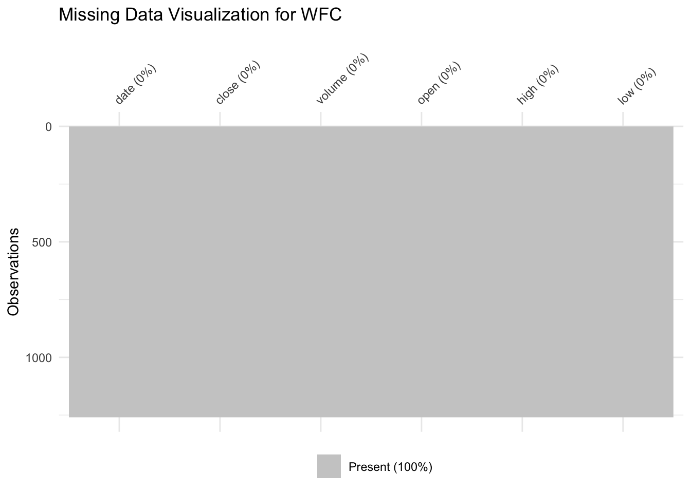

Code

# List of datasets
data_list <- list(BAC = BAC, GS = GS, JPM = JPM, MS = MS, WFC = WFC)

# Combine all datasets into one data frame with a 'Dataset' column indicating the dataset name
combined_data <- bind_rows(lapply(names(data_list), function(dataset_name) {
  data <- data_list[[dataset_name]]
  data$Dataset <- dataset_name
  return(data)
}))

# Convert all columns to character type
combined_data <- combined_data |>
  mutate(across(everything(), as.character))

# Pivot longer and add a column for missing data
combined_data_long <- combined_data |>
  pivot_longer(cols = -Dataset, names_to = "Column", values_to = "Value") |>
  mutate(Missing = is.na(Value))

# Plot the missing data across datasets
ggplot(combined_data_long, aes(x = Column, y = Dataset, fill = Missing)) +
  geom_tile(color = "white") +
  scale_fill_manual(values = c("TRUE" = "red", "FALSE" = "gray90")) +
  theme_minimal() +
  ggtitle("Missing Data Visualization Across Datasets") +
  theme(axis.text.x = element_text(angle = 45, hjust = 1))  # Rotate x-axis labels for better readability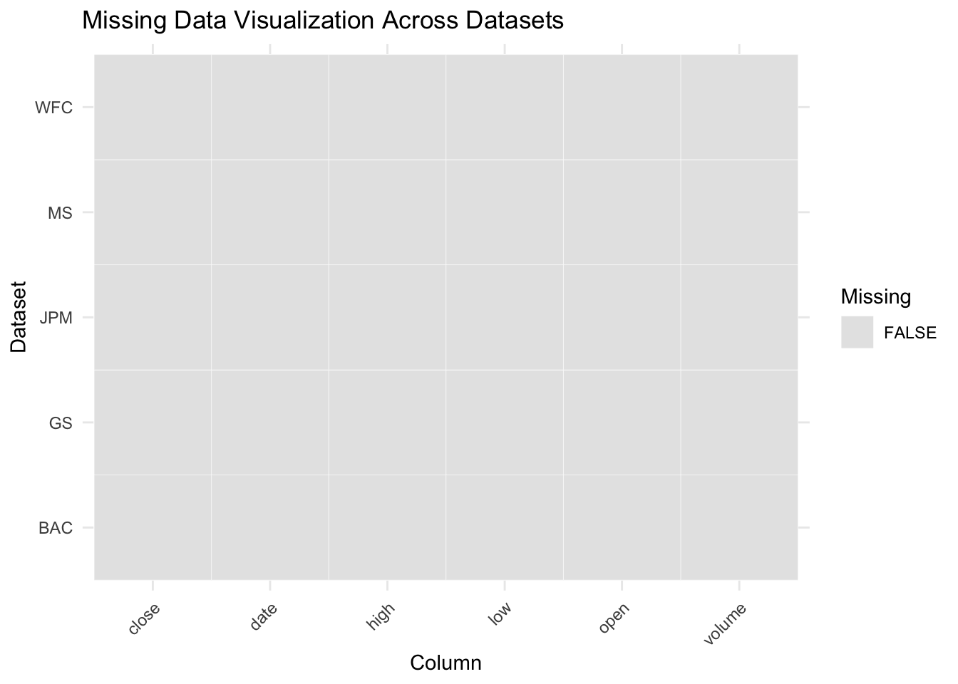

For the finance sector dataset, we have plotted two types of graphs:

A missing value heatmap for each company, which shows that there are no missing values across any column for each company. A comparative heatmap of the five companies in the finance sector, which confirms that none of the columns in any of the five datasets have missing values.

###Tech Sector

Fetching data

Code

#AAPL_history_data_url <- "https://api.nasdaq.com/api/quote/AAPL/historical?assetclass=stocks&fromdate=2019-11-20&limit=9999&todate=2024-11-20&random=21"
AAPL_csv_path <- "./Datasets/TECH/AAPL Historical data.csv"
#fetch_and_save_data(AAPL_history_data_url, AAPL_csv_path)


#GOOG_history_data_url <- "https://api.nasdaq.com/api/quote/GOOG/historical?assetclass=stocks&fromdate=2019-11-20&limit=9999&todate=2024-11-20&random=32"
GOOG_csv_path <- "./Datasets/TECH/GOOG class C Historical data.csv"
#fetch_and_save_data(GOOG_history_data_url, GOOG_csv_path)

# META_history_data_url <- "https://api.nasdaq.com/api/quote/META/historical?assetclass=stocks&fromdate=2019-11-20&limit=9999&todate=2024-11-20&random=13"
META_csv_path <- "./Datasets/TECH/GOOG class C Historical data.csv"
# fetch_and_save_data(GOOG_history_data_url, GOOG_csv_path)
 

# MSFT_history_data_url <- "https://api.nasdaq.com/api/quote/META/historical?assetclass=stocks&fromdate=2019-11-20&limit=9999&todate=2024-11-20&random=13"
MSFT_csv_path <- "./Datasets/TECH/MSFT Historical data.csv"
# fetch_and_save_data(MSFT_history_data_url, MSFT_csv_path)

# NVDA_history_data_url <- "https://api.nasdaq.com/api/quote/NVDA/historical?assetclass=stocks&fromdate=2019-11-20&limit=9999&todate=2024-11-20&random=49"
NVDA_csv_path <- "./Datasets/TECH/NVDA historical data.csv"
# fetch_and_save_data(NVDA_history_data_url, NVDA_csv_path)

Reading data

Code

aapl = read_csv(AAPL_csv_path)

Rows: 1259 Columns: 6
── Column specification ────────────────────────────────────────────────────────
Delimiter: ","
chr (5): date, close, open, high, low
num (1): volume

ℹ Use `spec()` to retrieve the full column specification for this data.
ℹ Specify the column types or set `show_col_types = FALSE` to quiet this message.

Code

goog = read_csv(GOOG_csv_path)

Rows: 1259 Columns: 6
── Column specification ────────────────────────────────────────────────────────
Delimiter: ","
chr (5): date, close, open, high, low
num (1): volume

ℹ Use `spec()` to retrieve the full column specification for this data.
ℹ Specify the column types or set `show_col_types = FALSE` to quiet this message.

Code

meta = read_csv(META_csv_path)

Rows: 1259 Columns: 6
── Column specification ────────────────────────────────────────────────────────
Delimiter: ","
chr (5): date, close, open, high, low
num (1): volume

ℹ Use `spec()` to retrieve the full column specification for this data.
ℹ Specify the column types or set `show_col_types = FALSE` to quiet this message.

Code

msft = read_csv(MSFT_csv_path)

Rows: 1259 Columns: 6
── Column specification ────────────────────────────────────────────────────────
Delimiter: ","
chr (5): date, close, open, high, low
num (1): volume

ℹ Use `spec()` to retrieve the full column specification for this data.
ℹ Specify the column types or set `show_col_types = FALSE` to quiet this message.

Code

nvda = read_csv(NVDA_csv_path)

Rows: 1259 Columns: 6
── Column specification ────────────────────────────────────────────────────────
Delimiter: ","
chr (5): date, close, open, high, low
num (1): volume

ℹ Use `spec()` to retrieve the full column specification for this data.
ℹ Specify the column types or set `show_col_types = FALSE` to quiet this message.

Code

#missing data
datasets <- list(
  "AAPL" = aapl,
  "GOOG" = goog,
  "META" = meta,
  "MSFT" = msft,
  "NVDA" = nvda
)

for (name in names(datasets)) {
  cat(paste("Missing values in", name, "dataset:\n"))
  print(colSums(is.na(datasets[[name]])))
  cat("\n")
}

Missing values in AAPL dataset:
  date  close volume   open   high    low 
     0      0      0      0      0      0 

Missing values in GOOG dataset:
  date  close volume   open   high    low 
     0      0      0      0      0      0 

Missing values in META dataset:
  date  close volume   open   high    low 
     0      0      0      0      0      0 

Missing values in MSFT dataset:
  date  close volume   open   high    low 
     0      0      0      0      0      0 

Missing values in NVDA dataset:
  date  close volume   open   high    low 
     0      0      0      0      0      0

Code

#missing values visualisation
#install.packages('naniar')
#install.packages('VIM')
#library(dplyr)
#library(tidyverse)
#library(ggplot2)
#library(naniar)

# Assuming the files are named file1, file2, ..., file5
aapl$Source <- "Apple"
goog$Source <- "Google"
meta$Source <- "Meta"
msft$Source <- "Microsoft"
nvda$Source <- "Nvidia"

# Combine the datasets
all_files <- bind_rows(aapl, goog, meta, msft, nvda)

# Reshape data for visualization
# Create a missingness indicator for each column
all_files <- all_files  |> 
  mutate(across(-Source, as.character))

# Pivot the data
missing_long <- all_files  |> 
  pivot_longer(cols = -Source, names_to = "Variable", values_to = "Value")  |> 
  mutate(Missing = is.na(Value))
library(ggplot2)

ggplot(missing_long, aes(x = Variable, y = Source, fill = Missing)) +
  geom_tile(color = "white") +
  scale_fill_manual(
    values = c("TRUE" = "red", "FALSE" = "blue"),
    labels = c("TRUE" = "Missing", "FALSE" = "Not Missing")
  ) +
  theme_minimal() +
  labs(
    title = "Missing Data Across Files",
    x = "Variables",
    y = "Files",
    fill = "Missing?"
  ) +
  theme(axis.text.x = element_text(angle = 90, hjust = 1))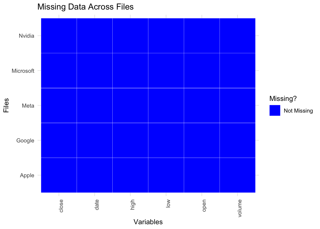

There are 2 of types visualizations we have done to depict the missing values in the data.One using regular ggplot and the other using the naniar package.As seen from the graphs, there are no missing values.This trend can be attributed to the fact that all stocks have a price and they are updated accordingly. To deal with historical data, NASDAQ would probably use multiple techniques like archival techniques and curation processes etc. Another widely known fact is that financial data is almost always very clean.

###Healthcare and Pharma Sector

Fetch Data:

Code

# JNJ_history_data_url <- "https://api.nasdaq.com/api/quote/JNJ/historical?assetclass=stocks&fromdate=2019-11-20&limit=9999&todate=2024-11-20&random=45"
JNJ_csv_path <- "./Datasets/Healthcare and Pharma/JNJ Historical data.csv"
# fetch_and_save_data(JNJ_history_data_url, JNJ_csv_path)
# 
# 
# AZN_history_data_url <- "https://api.nasdaq.com/api/quote/AZN/historical?assetclass=stocks&fromdate=2019-11-20&limit=9999&todate=2024-11-20&random=20"
AZN_csv_path <- "./Datasets/Healthcare and Pharma/AZN Historical data.csv"
# fetch_and_save_data(AZN_history_data_url, AZN_csv_path)
# 
# 
# LLY_history_data_url <- "https://api.nasdaq.com/api/quote/LLY/historical?assetclass=stocks&fromdate=2019-11-20&limit=9999&todate=2024-11-20&random=22"
LLY_csv_path <- "./Datasets/Healthcare and Pharma/LLY Historical data.csv"
# fetch_and_save_data(LLY_history_data_url, LLY_csv_path)
# 
# MRK_history_data_url <- "https://api.nasdaq.com/api/quote/MRK/historical?assetclass=stocks&fromdate=2019-11-20&limit=9999&todate=2024-11-20&random=33"
MRK_csv_path <- "./Datasets/Healthcare and Pharma/MRK Historical data.csv"
# fetch_and_save_data(MRK_history_data_url, MRK_csv_path)
# 
# PFE_history_data_url <- "https://api.nasdaq.com/api/quote/PFE/historical?assetclass=stocks&fromdate=2019-11-20&limit=9999&todate=2024-11-20&random=49"
PFE_csv_path <- "./Datasets/Healthcare and Pharma/PFE Historical data.csv"
# fetch_and_save_data(PFE_history_data_url, PFE_csv_path)

Reading Data:

Code

# Reading the datasets using relative paths
jnj = read_csv(JNJ_csv_path)

Rows: 1259 Columns: 6
── Column specification ────────────────────────────────────────────────────────
Delimiter: ","
chr (5): date, close, open, high, low
num (1): volume

ℹ Use `spec()` to retrieve the full column specification for this data.
ℹ Specify the column types or set `show_col_types = FALSE` to quiet this message.

Code

azn = read_csv(AZN_csv_path)

Rows: 1259 Columns: 6
── Column specification ────────────────────────────────────────────────────────
Delimiter: ","
chr (5): date, close, open, high, low
num (1): volume

ℹ Use `spec()` to retrieve the full column specification for this data.
ℹ Specify the column types or set `show_col_types = FALSE` to quiet this message.

Code

lly = read_csv(LLY_csv_path)

Rows: 1259 Columns: 6
── Column specification ────────────────────────────────────────────────────────
Delimiter: ","
chr (5): date, close, open, high, low
num (1): volume

ℹ Use `spec()` to retrieve the full column specification for this data.
ℹ Specify the column types or set `show_col_types = FALSE` to quiet this message.

Code

mrk = read_csv(MRK_csv_path)

Rows: 1259 Columns: 6
── Column specification ────────────────────────────────────────────────────────
Delimiter: ","
chr (5): date, close, open, high, low
num (1): volume

ℹ Use `spec()` to retrieve the full column specification for this data.
ℹ Specify the column types or set `show_col_types = FALSE` to quiet this message.

Code

pfe = read_csv(PFE_csv_path)

Rows: 1259 Columns: 6
── Column specification ────────────────────────────────────────────────────────
Delimiter: ","
chr (5): date, close, open, high, low
num (1): volume

ℹ Use `spec()` to retrieve the full column specification for this data.
ℹ Specify the column types or set `show_col_types = FALSE` to quiet this message.

Code

pharma_datasets <- list(
  "JNJ" = jnj,
  "AZN" = azn,
  "LLY" = lly,
  "MRK" = mrk,
  "PFE" = pfe
)

for (name in names(pharma_datasets)) {
  cat(paste("Missing values in", name, "dataset:\n"))
  print(colSums(is.na(pharma_datasets[[name]])))
  cat("\n")
}

Missing values in JNJ dataset:
  date  close volume   open   high    low 
     0      0      0      0      0      0 

Missing values in AZN dataset:
  date  close volume   open   high    low 
     0      0      0      0      0      0 

Missing values in LLY dataset:
  date  close volume   open   high    low 
     0      0      0      0      0      0 

Missing values in MRK dataset:
  date  close volume   open   high    low 
     0      0      0      0      0      0 

Missing values in PFE dataset:
  date  close volume   open   high    low 
     0      0      0      0      0      0

Missing Values Visualisation

Code

# Assuming the files are named file1, file2, ..., file5
jnj$Source <- "JNJ"
azn$Source <- "AstraZeneca"
lly$Source <- "Eli Lilly"
mrk$Source <- "Merck&Co"
pfe$Source <- "Pfizer"

# Combine the datasets
all_files_health <- bind_rows(jnj, azn, lly, mrk, pfe)

# Reshape data for visualization
# Create a missingness indicator for each column
all_files_health <- all_files_health  |> 
  mutate(across(-Source, as.character))

# Pivot the data
missing_long <- all_files_health  |> 
  pivot_longer(cols = -Source, names_to = "Variable", values_to = "Value")  |> 
  mutate(Missing = is.na(Value))
library(ggplot2)
library(naniar)

gg_miss_var(all_files_health, facet = Source) +
  theme(axis.text.x = element_text(angle = 45, hjust = 1)) +
  labs(title = "Missing Data Visualization by File")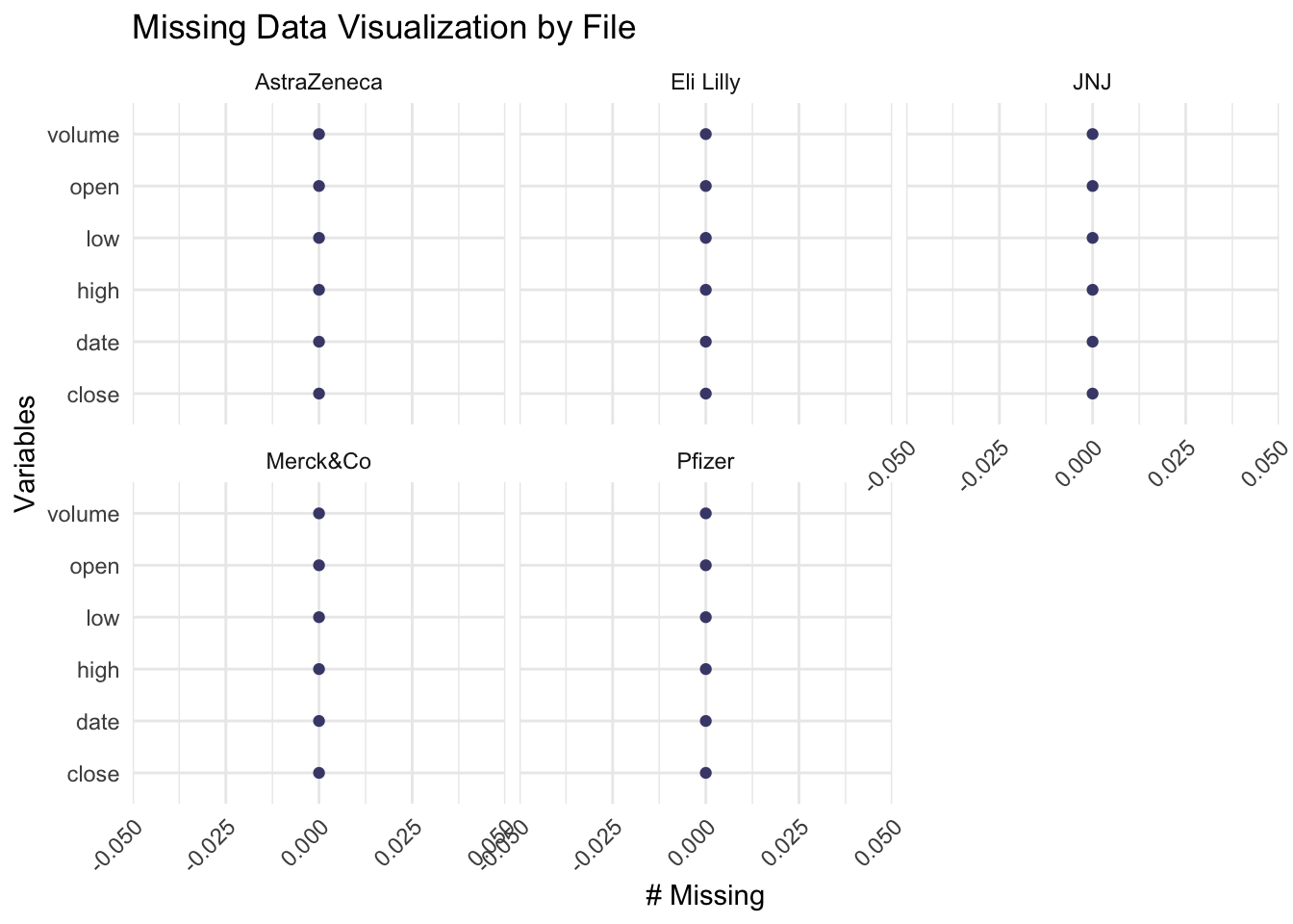

We have used naniar package to visualise missing data. The x-axis shows the proportion of data missing in the dataset and here since its 0, it means there are no missing values. The reason why has been explained above.

There are 3 of types visualizations we have done to depict the missing values in the data. Two using regular ggplot and the other using the naniar package. As seen from the graphs, there are no missing values.This trend can be attributed to the fact that all stocks have a price and they are updated accordingly. To deal with historical data, NASDAQ would probably use multiple techniques like archival techniques and curation processes etc. Another widely known fact is that financial data is almost always very clean.